本次美国代写是matlab数字信号处理的一个Lab
A note before starting
A Fourier Series is a series of sinusoidal functions added together to approximate a time-based signal. The sinusoidal functions differ in their frequencies and may differ in their amplitudes. DO NOT confuse a Fourier
Series with a Fourier Transform. A Fourier Transform is the transformation of a signal from the time domain to the frequency domain. This lab will focus on Fourier Series and introduce you to Fourier Transforms.
PART 1: IMPLEMENTING A FOURIER SERIES (40 PTS)
The following function creates a periodic square wave:
function f = periodicSquare(t, tau)
tprime = mod(t+pi,2*pi) – pi;
y = (tprime > -tau/2) & (tprime < tau/2);
f=double(y); %force logical to double
end
The input t is a time vector and the input τ alters the square wave.
1. Create a time vector ranging from -10 to 10 with a sufficiently fine resolution. Using the subplot command, create a 4×1 figure in which you plot y vs. t for 𝜏𝜏 =𝜋/2, 𝜋, 3𝜋/2, and 2𝜋. (5 pts)
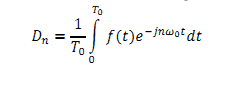
2. By hand, calculate the exponential Fourier Series coefficients, D and D , of the periodic square wave in terms of n and τ. Type your results, step-by-step, into your lab report using the Equation Editor or Math Type in Microsoft Word. Recall the equation for these coefficients:
3. What is the effect of τ in shaping this waveform? What is the period of each waveform? (5 pts)