本次加拿大代写是R数值模拟的一个assignment
In this first assignment, I want you to analyze the properties of a few estimators. I want you to create a Rmd file, compile it and upload both the Rmd and PDF files before Sunday October 3 at 10:00pm. I usually do not answer emails during the weekend, so do not start at the last minute in case you need help. You are allowed to discuss with each other, but I expect each copy to be unique.
If some simulations are too long to compile, you can generate the solution and save it into an .Rda file and load the file in your document to present the result. This will make it easier for you to compile the PDF. If you choose to proceed this way, include the code for the simulation with the option eval=FALSE. Here is an example. You first show the simulation code without running it (you can run it once on your side to get the result):
Xvec <- numeric()
for (i in 1:10000)
{
x <- rnorm(5000)
Xvec[i] <- mean(x)
}
save(Xvec, file=”A1Res.rda”)
Then, you print the result:
load(“A1Res.rda”)
mu <- mean(Xvec)
rmse <- sqrt(mean(Xvecˆ2))
rmse
## [1] 0.01405928
If you use this method, upload all .rda files needed to compile the PDF.
Important: Before you start any simulation, set the seed to your student number. Also, set the number of iterations to 2,000 for all your simulations.
Estimator of the covariance
We saw that the unbiased estimator of the variance, S2, is less efficient than ˆ σ2 = (n − 1)S2/n. We also sawin a simulation that the RMSE of ˆ σ2 is smaller. In this question, we want to see if we get the same result for the following estimators of the covariance:
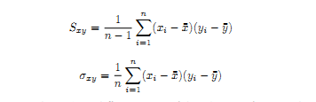
Set the sample size to n = 25 and try three different pairs of distributions for X and Y . For each pair, report the RMSE of both estimators. Interpret your result.
Estimator of the mean for non-identically distributed samples.
We saw that ¯ X is the best linear unbiased estimator of the mean, which means that it is has the smallest variance among all estimators that can be defined as:

However, this is true only for iid samples. In your simulation, consider a sample of 100 observations with xi ∼ iid(0, σ2
1) for i = 1, …, 50 and xi ∼ iid(0, σ2
2) for i = 51, …, 100.
• In the first simulation, compare the bias, standard error and RMSE for ¯ X and ˆ µ using wi = 1/σ2 for i = 1, …, 50 and wi = 1/σ2
2 for i = 51, …, 100. We also assume that σ2
i ’s are known. You can try a few distributions and see if it affects the properties.
• In the second simulation, we use the same weights but we assume that the σ2
i ’s are unknown. Therefore, we replace them by estimators. Since it is a different estimator, we call it ˜ µ. Using the same realized samples as in the previous simulation, compare the bias, standard error and RMSE of ˜ µ and ¯ x.
Do we see a difference when the true variances are replaced by estimates? Explain.